Here’s a trick I use in Numbers all of the time—hiding rows to better see what I’m doing. So for example, let’s say I have this spreadsheet. I mean, I do have this spreadsheet, but let’s say I do, too.
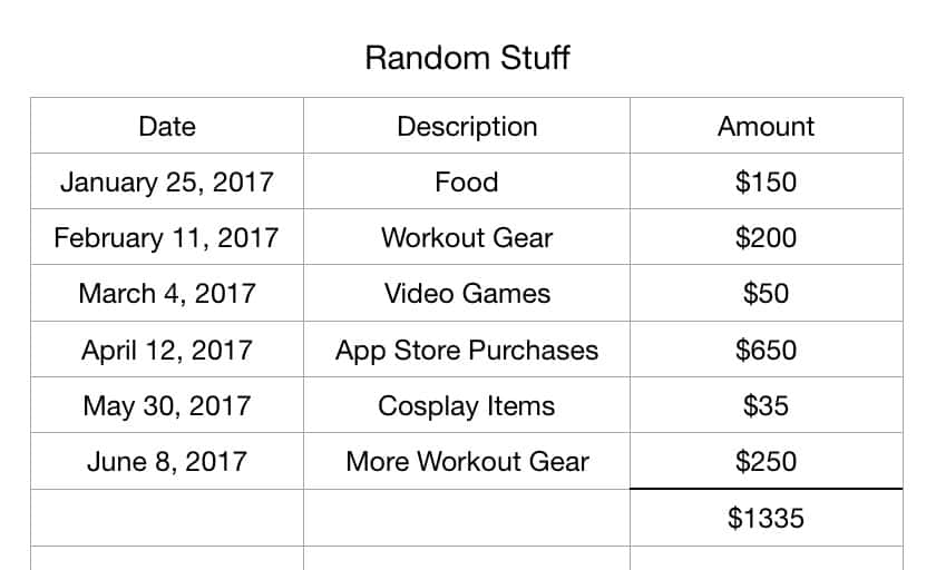
Those amounts aren’t real, guys. At least, most of them aren’t.
So in a spreadsheet like this, if you keep on entering row after row of data, eventually you’re going to get tired of scrolling down to get to the next blank line. One way to make this simpler is by designating a header row—if the template you’re using doesn’t have one included automatically, you can hover over the number next to your header row to reveal an arrow…
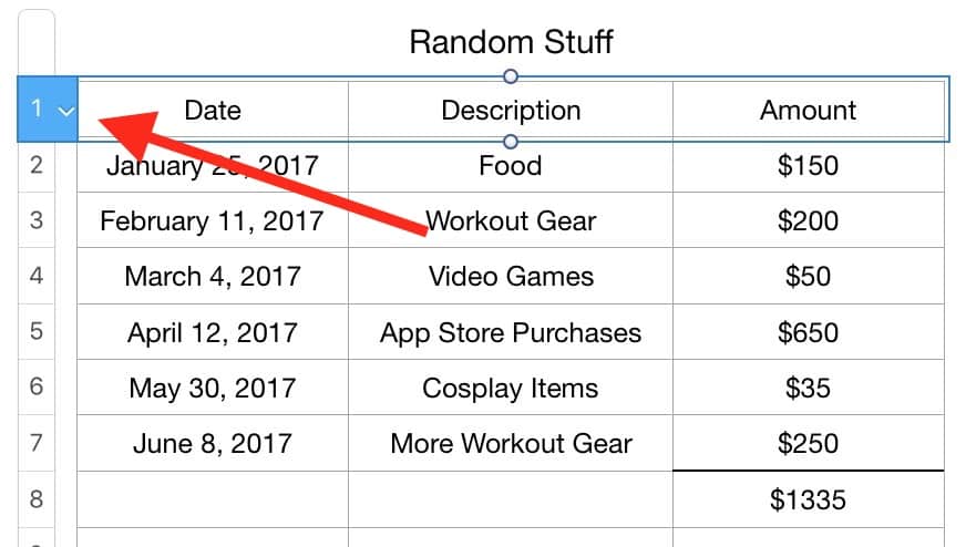
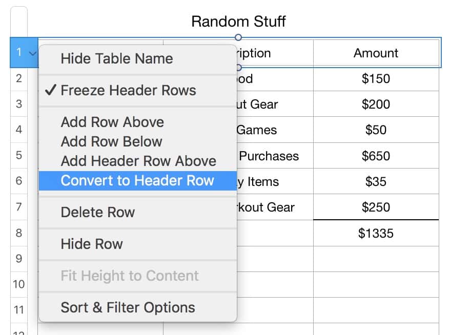
…and then when you click the arrow, a contextual menu will appear with the “Convert to Header Row” option.
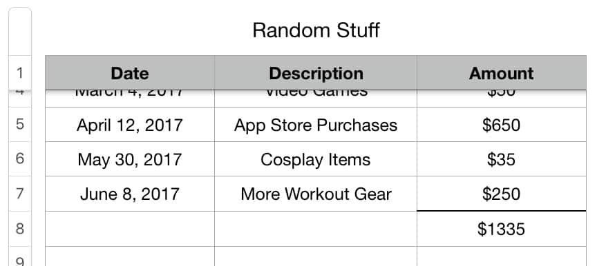
The benefit of this is that when you scroll up and down, your header will stay put, making it easy to see where you’re supposed to be entering info.
As I mentioned, though, the way I like to handle this is by hiding rows I’ve already finished entering data into. You see, I’m usually concerned with the totals, not the individual item details, so it makes sense just to focus on the most relevant entries without having fifty million rows to scroll past. Here’s how you do that! First, click and drag on the row numbers to select the ones you’d like to hide.
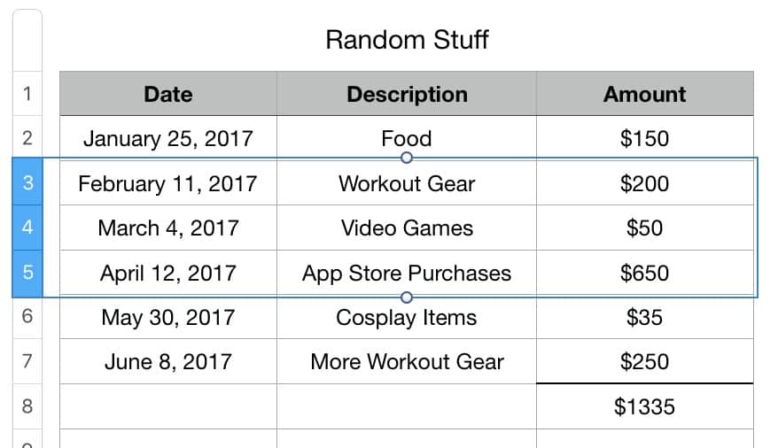
Then you can either hover over and click the arrow I mentioned above on any of the selected rows, or you could right-click anywhere within the selection. Either way, you’ll pick “Hide Selected Rows” from the choices.
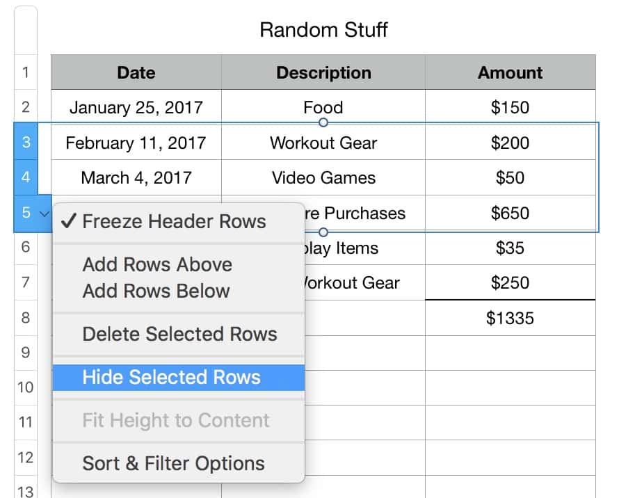
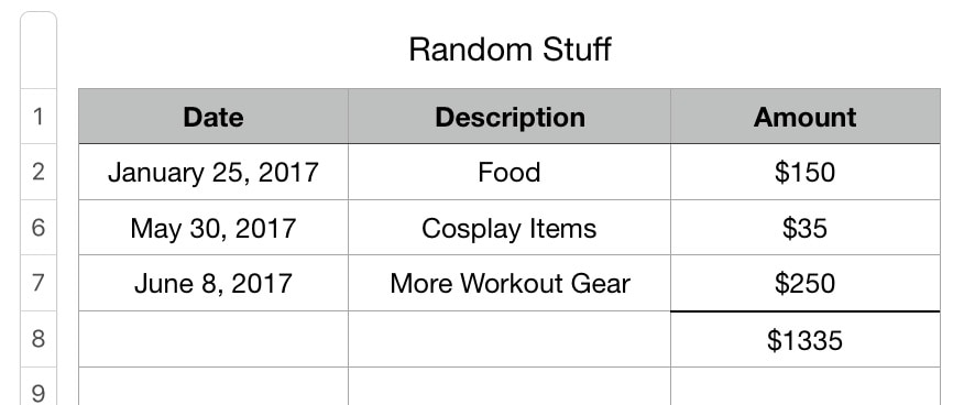
Then—voilà—those rows will vanish, but they’ll still affect the column totals, of course.
If you’d like to unhide your rows, you can use the arrows again:
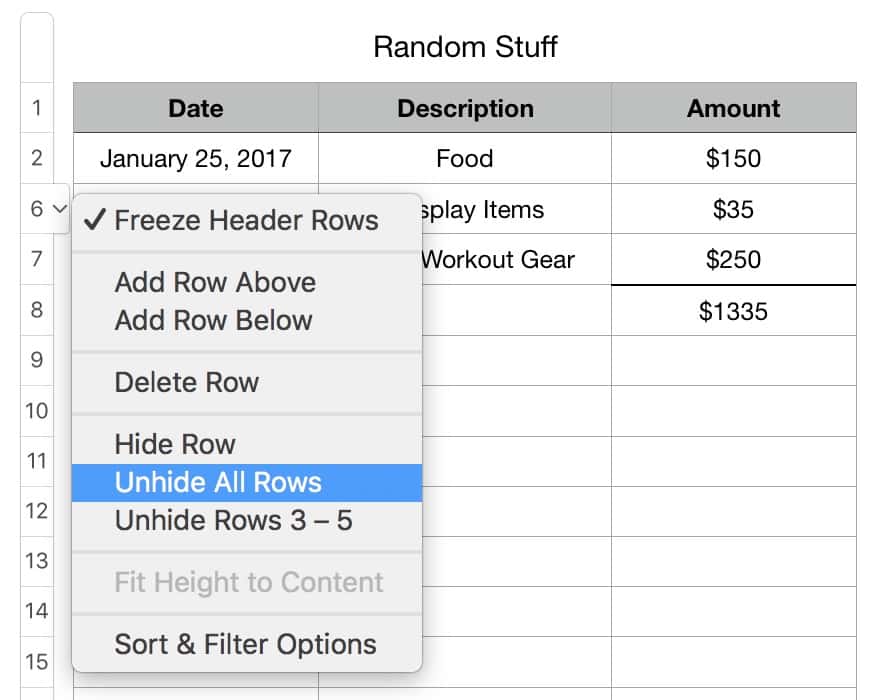
Or you could employ the “Table” menu at the top of your screen.
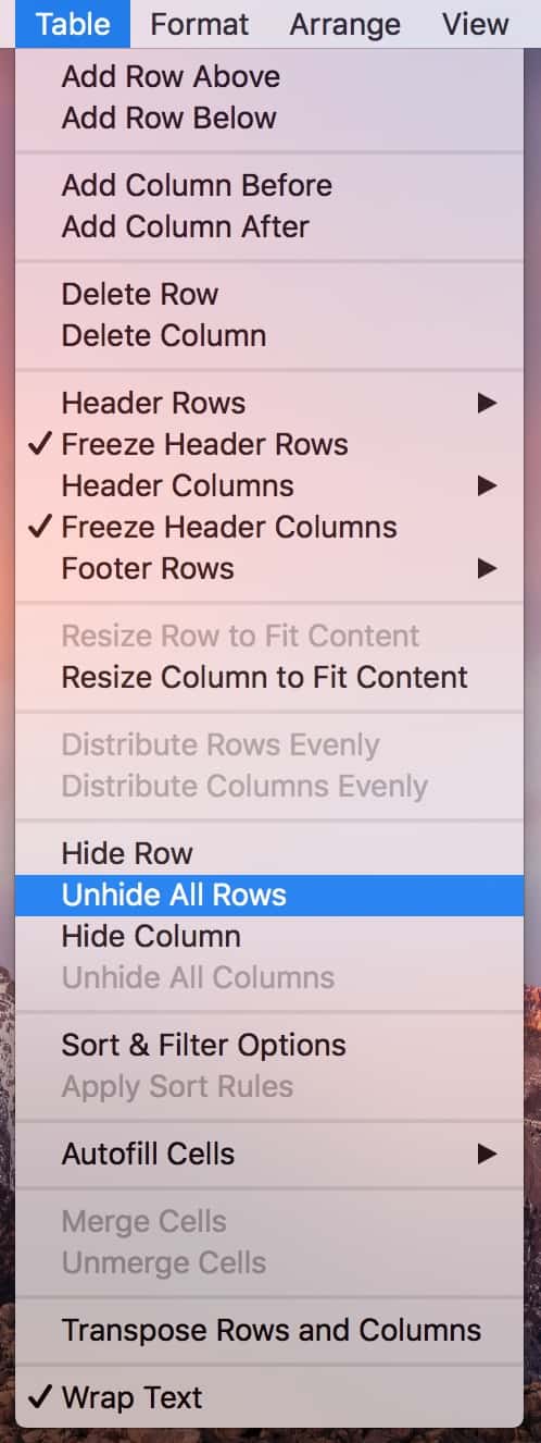
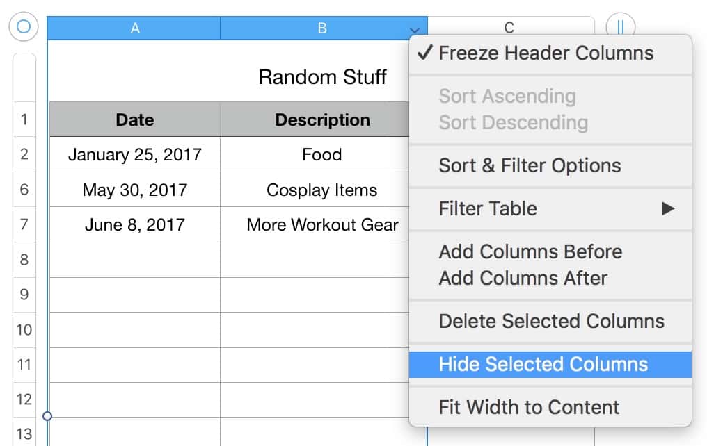
I have a few additional notes here. First, know that you can hide columns, too, with very similar steps. I find this much less useful, but you’re not me, so maybe you’ll like this.
Also, this same feature is available in Microsoft Excel. An easy way to use it is by selecting the rows or columns you want to hide (by dragging across their numbers or letters) and then going under the “Format” menu.
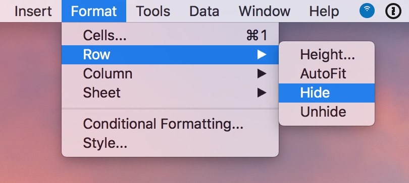
As you can see, “Unhide” is there as well when you’re ready to show all of your data again (but be sure you’ve selected the rows bordering the hidden ones first).
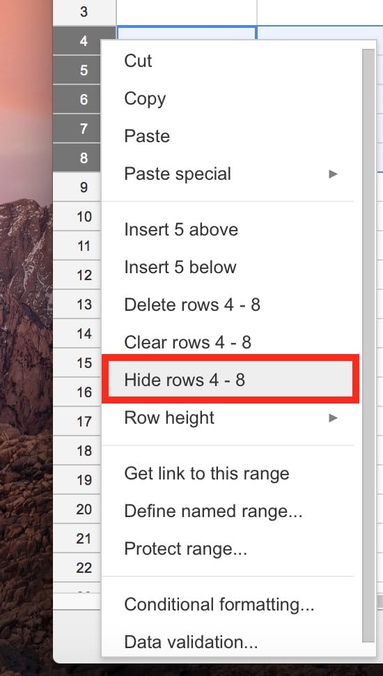
If what you’re using is Google Sheets, you’ll do this same thing by selecting the rows to hide, then right- or Control-clicking on any of the numbers that designate them. This’ll reveal a menu from which to pick “Hide rows.”
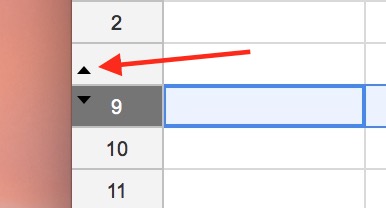
Sheets will then helpfully add some arrows within the row numbers to indicate that there’s a hidden section, and you could click those to reveal everything once again.
Whew! Hope this is useful information for you. I use Numbers on a daily basis for all sorts of business-related tracking, so even though it makes me feel a little nuts to say this, it’s one of my favorite programs!
God, I am so boring. Send help.
Great tip! I use Numbers as my checkbook register and by this time of the year there can be quite a few rows.